Calculate ocean pCO2 and pH from DIC, alkalinity, and temperature
Seawater properties
MODEL DESCRIPTION
This web app calculates the partial pressure of CO\(_2\) (pCO\(_2\)) and pH of seawater in equilbrium with the atmosphere given sea-surface temperature, titration alkalinity, and dissolved inorganic carbon.
The calculation is based on simplified carbonate equilibria including dissolved CO\(_2\), bicarbonate ion [HCO\(_{3}^-\)], carbonate ion [CO\(_{3}^{2-}\)], hydrogen ion [H\(^+\)], and borate [HBO\(_3^-\)]. Both phosphate [PO\(_4^{3-}\)] and silicic acid H\(_{2}\) SiO\(_4\) are neglected. The simplification is intended to represent large-scale mean conditions and is probably not accurate to better than about 1 ppmv of pCO\(_2\).
The model is based on a discussion in an article by Pieter Tans (1996). You can read all the gory details in the “Chemistry” tab to the right of this one.
The program that does the calculation is very simple, and the code that controls this website is surprisingly simple too! It is all written in the programming language R, using a web programming package called shiny. You can read all about it on the “Website Code” tab to the right.
Simplified Carbonate Chemistry of Seawater
The discussion below is based on an article by Pieter Tans (1998). Readers interested in a more in-depth presentation might want to refer to classic textbooks by Sarmiento and Gruber (2006, Chapters 8-10) or Williams and Follows (2011, Chapter 6).
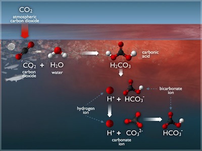
Dissolved carbon dioxide in water forms carbonic acid (H2CO3), which dissociates twice to form protons (H+), bicarbonate (HCO3-) and carbonate (CO32-) ions in solution. In equilibrium, we have
\[ \begin{array}{lclcr} CO_2(g) & \rightleftharpoons & CO_2(aq) & K_0 = \frac{[CO_2 (aq)]}{pCO_2} & (1)\ CO_2(aq) + H_2O & \rightleftharpoons & H^+ + HCO_3^- & K_1 = \frac{[HCO_3^-][H^+]}{[CO_2 (aq)]} & (2) \ HCO_3^- & \rightleftharpoons & H^+ + CO_3^{2-} & K_2 = \frac{[CO_3^{2-}][H^+]}{HCO_3^-} & (3) \ \end{array} \]
The equilibria in (1) through (3) provide a system of three equations in five unknowns (pCO\(_2\), [CO\(_2\)(aq)], [HCO\(_3^-\)], [CO\(_3^{2-}\)], and [H\(^+\)] or pH). To solve, we need two additional constraints. We add additional equations for titration alkalinity (TA) and total dissolved inorganic carbon (DIC), both of which are commonly measured:
\[ \begin{array}{lclr} DIC & = & [CO_2(aq)] + [HCO_3^-] + [CO_3^{2-}] & (4) \ TA & = & [HCO_3^-] + 2 [CO_3^{2-}] + [B(OH)_4^-] + [OH^-] - [H^+] \pm [minor\ species] & (5) \end{array} \]
In some areas of the ocean, we have to be more inclusive in specifying alkalinity to include nitrate, phosphate, and silica. This is especially important where there's a lot of biology. According to Follows et al (2006), neglecting these species typically leads to errors in pCO\(_2\) of order 1 ppmv, so we'll just stick with the simpler formulation here.
In most cases, the alkalinity is made up almost entirely of the bacarbonate and carbonate anions, whose sum is sensibly called the “carbonate alkalinity (CA).” But since we can't directly measure CA, it's usually calculated by subtracting the minor ions from the (measured) TA.
In (5), [B(OH)\(_4^-\)] is the concentration of the borate ion produced by the dissociation of Boric acid (B(OH)\(_3\), and yes, this is the stuff your mother used to put in your eyes). Uh oh! Now we've introduced yet another unknown (borate), so we have to add yet another constraint as well. But this is no big deal.
It turns out that the element-by-element composition of sea salt is almost perfectly identical everywhere in the sea, though it's more dilute in some places than and more concentrated (“saline”“) in others. So it's easy to know the total amount of Boron in the water if we just know the salinity.
The total Boron in any seawater sample is a fixed fraction of the salinity, so
[Boron] = [B(OH)\(_3\)] + [B(OH)\(_4^-\)] = 1.179 x 10\(^{-5}\) S, where S = 34.78 permil and [Boron] is in mol kg\(^{-1}\).
Boric acid dissociation can also be written as an equilibrium \[ \begin{array}{lclcr} B(OH)_3 & \rightleftharpoons & H^+ + B(OH)_4^- & K_B = \frac{[B(OH)_4^-][H^+]}{[B(OH)_3]}&(6) \end{array} \]
Believe it or not, we've now got 6 equations (1) - (6) in six unknowns! The equilibrium coefficients K\(_0\), K\(_1\), K\(_2\), and K\(_B\) have all been measured very accurately as functions of temperature and salinity, and just get plugged into the equations as "constants.” We use the values from the Tans chapter (his Table 12.1) here. You can read or copy/paste the R code by clicking the Website Code tab to the right.
To solve the carbonate system, we first use (1), (2), and (3) to write
\[ \begin{array}{lclr} DIC & = & (1 + \frac{K_1}{[H^+]} + \frac{K_1 K_2}{[H^+]^2}) [CO_2(aq)] & (7)\ CA & = & (\frac{K_1}{[H^+]} + \frac{2 K_1 K_2}{[H^+]^2}) [CO_2(aq)] & (8)\ \end{array} \]
Dividing (7) by (8) gives a quadratic for [H\(^+\)]: \[ \begin{array}{lclr} (CA)[H^+]^2 + K_1(CA - DIC)[H^+] + K_1 K_2 (CA - 2 DIC) = 0. & (9) \end{array} \]
Finally, we use the definitions of CA and TA, and the boric acid equilibrium (6) to write \[ \begin{array}{lclr} CA & = & TA - \frac{K_B}{(K_B + [H^+])}[Boron] & (10) \end{array} \]
Starting with DIC and TA and a “first guess” of pH = 8, we solve (10) for CA, then substitute the value into (9) and solve the quaratic for a new estimate of [H\(^+\)]. Then we iterate equations (10) and (9) until the resulting estimates of [H\(^+\)] converge.
Once the iteration converges, we just substitute the value of [H\(^+\)] back into (1), (2), and (3) to obtain [CO\(_3^{2-}\)], [HCO\(_3^-\)], [CO\(_2\)(aq)], and pCO\(_2\).
It is also useful to calculate the “Revelle buffer factor,” which is approximately
\[ R = \frac{DIC}{[CO_3^{2-}]}. \]
The Revelle factor indicates the fractional change in pCO\(_2\) per fractional change in DIC, and is about 10 for current global mean conditions. This means that doubling atmospheric pCO\(_2\) (a 100% increase) would lead to only a 10% increase in marine DIC.
The iterative solution and then backsubstitution is a lot simpler than it sounds. To read the code, click the “Website Code” tab to the right.
References Cited
P. Tans, “Why Carbon Dioxide from Fossil Fuel Burning Won't Go Away” In: MacAladay, J. (ed), “Environmental Chemistry,” Oxford University Press, 1998. pp. 271-291.
Williams, R. G. and M. J. Follows, Ocean Dynamics and the Carbon Cycle. Cambridge University Press, 2011. Order from Amazon
Sarmiento, J. L. and N. Gruber, 2006. Ocean Biogeochemical Dynamics. Princeton University Press, 2006.
Follows, M. J., T. Ito, and S. Dutkiewicz (2006), On the solution of the carbonate chemistry system in ocean biogeochemistry models, Ocean Modelling, 12(3-4), 290–301, doi:10.1016/j.ocemod.2005.05.004.
How this website works (including all the code!)
This website is controlled using the R package “shiny.” There are three important components:
- A script (carbonate.R) that performs the simple carbonate equilibrium calculations
- The user interface (ui.R) that controls the sliders and passes inputs to the model
- The “server” (server.R) that responds to user interface events in the web browser
Scroll down or click links in the list above to read all about it!
carbonate.R:
carbonate = function(TEMP=16., alk=2311, DIC=2002, pH=8.) {

# Carbonate equilibrium system based on
# P. Tans, "Why Carbon Dioxide from Fossil Fuel Burning Won't Go Away"
#  In: MacAladay, J. (ed),  "Environmental Chemistry," 1996. pp.

# Note that we are ignoring contributions of PO4 and SiO4 to alkalinity, which may be
# important regionally but probably lead to errors in pCO2 < 1 ppmv globally
# See Follows et al (2006) for a discussion of this approximation

# Default values if the user doesn't specify at runtime are for preindustrial global surface

# Tans defines pCO2 via Henry's Law in atmospheres
# I'm converting to ppmv for clarity
#
# Variable definitions

# INPUT VARIABLES
#       T      #  Temperature (Celsius)
#       TA     #  titration alkalinity (equivalents/kg)
#       DIC    #  total dissolved inorganic carbon (mol/kg)

# OUTPUT VARIABLES
#       pH     #  pH of the water (-log(H))
#       pCO2    #  partial pressure of CO2 (Pascals)
#       iter   iteration count

# CHEMICAL & THERMODYNAMIC COEFFICIENTS
#       K0     #  Henry's Law constant
#       K1     #  first dissociation coefficient for H2CO3
#       K2     #  second dissociation coefficient for H2CO3
#       Kb     #  dissociation constant for boric acid
#       S      #  Salinity (g/kg)
#       Boron  #  total boron (mol/kg)
#       H0     #  "old" concentration of hydrogen ion (mol/kg)

# INTERNAL VARIABLES USED TO CALCULATE pCO2 and pH
#       H      #  current concentration of hydrogen ion (mol/kg)
#       CA     #  carbonate alkalinity (eq / l)
#       CO2aq  #  concentration of aqueous CO2
#       diff.H  #  difference in successive estimates of H+ (mol/kg)
#       tiny.diff.H   (1e-15) test for convergence
#       a      #  first term in quadratic for eq 12
#       b      #  second term in quadratic for eq 12
#       c      # third term in quadratic for eq 12

# Convert input units to mks
TEMP <- TEMP + 273.15 # temperature from Celsius to Kelvin
alk <- alk * 1.e-6    # microequivalents to equivalents
DIC <- DIC * 1.e-6    # micromoles to moles

# Set values of prescribed constants
S <- 34.78                 # Salinity in ppt
Boron <- 1.179e-5 * S      # Total Boron mole/kg as a fraction of salinity

# Carbonate and boric acid equilibrium constants as functions of temp and S
K0 <- exp(-60.2409 + 9345.17/TEMP + 23.3585*log(TEMP/100)
          + S * (0.023517 - 0.00023656*TEMP +0.0047036*(TEMP/100)^2) )

K1 <- exp(2.18867 - 2275.036/TEMP - 1.468591 * log(TEMP)
          + (-0.138681 - 9.33291/TEMP) * sqrt(S) + 0.0726483*S
          - 0.00574938 * S ^1.5)

K2 <- exp(-0.84226 - 3741.1288/TEMP -1.437139 * log(TEMP)
          + (-0.128417 - 24.41239/TEMP)*sqrt(S) + 0.1195308 * S
          - 0.0091284 * S ^1.5 )

Kb <- exp( (-8966.90 - 2890.51*sqrt(S) - 77.942*S
            + 1.726 * S ^1.5 - 0.0993*S^2) / TEMP
            + (148.0248 + 137.194 * sqrt(S) + 1.62247 * S)
            + (-24.4344 - 25.085 * sqrt(S) - 0.2474 * S) * log(TEMP)
            + 0.053105 * sqrt(S) * TEMP)

# Iterate for H and CA by repeated solution of eqs 13 and 12
H <- 10.^(-pH)                 # initial guess from arg list
diff.H <- H
tiny.diff.H <- 1.e-15

iter <- 0

while (diff.H > tiny.diff.H) {     # iterate until H converges

  H.old <- H                      # remember old value of H

  # solve Tans' equation 13 for carbonate alkalinity from TA
  CA <- alk - (Kb/(Kb+H)) * Boron

  # solve quadratic for H (Tans' equation 12)
  a <- CA
  b <- K1 * (CA - DIC)
  c <- K1 * K2 * (CA - 2 * DIC)
  H <- (-b + sqrt(b^2 - 4. * a * c) ) / (2. * a)

  # How different is new estimate from previous one?
  diff.H <- abs(H - H.old)
  iter <- iter + 1

}

# Now solve for CO2 from equation 11 and pCO2 from eq 4
CO2aq <- CA / (K1/H + 2*K1*K2/H^2)  # Eq 11
pCO2 <- CO2aq / K0 * 1.e6           # Eq 4 (converted to ppmv)
pH <- -log10(H)

return(list(TEMP=TEMP-273.15, alk=alk*1.e6, DIC=DIC*1.e6, pH=pH, pCO2=pCO2, iter=iter))
}
This is the user interface that actually controls this website
ui.R:
library(shiny)
library(markdown)

# Define UI for seawater carbonate application
shinyUI(pageWithSidebar(

  #  Application title
  headerPanel("Calculate ocean pCO2 and pH from DIC, alkalinity, and temperature"),

  # Sidebar with sliders that demonstrate various available options
  sidebarPanel(
    selectInput("scenario", "Scenario:", selected='preindustrial',
                list("Preindustrial" = "preindustrial",
                     "Modern" = "modern",
                     "Glacial" = "glacial",
                     "Custom" = "custom")),
    h4('Set Seawater Parameters'),
    sliderInput('alk', 'Titration Alkalinity (microequivalents per kg)',
                min = 2000, max = 2500, value = 2311, step= 1),

    sliderInput('sst', 'Temperature (Celsius)',
                min = -2, max = 34, value = 16, step= 0.1),

    sliderInput('dic', 'Dissolved Inorganic Carbon (micromoles per kg)',
                min = 1900, max = 2200, value = 2002, step=1)
   ),

   # Main panel consists of a tabset displays model output or model description
   mainPanel(
     tabsetPanel(
       tabPanel('Results',
                h4('Seawater properties'),
                img(src='diagram.jpg', align='right'),
                tableOutput('summary'),
                plotOutput('bjerrum')),
       tabPanel('Description',
                includeHTML('doc/model.description.html')),
       tabPanel('Chemistry',
                includeHTML('doc/chemistry.html')),
       tabPanel('Website Code',
                includeMarkdown('doc/website.code.md'))
     )
  )
))
server.R:
library(shiny)

# Source required R scripts
source('model/carbonate.R')
source('model/report.output.R')
source('model/plot.bjerrum.R')

shinyServer(function(input, output, session) {

  # Read preset scenarios from a file
  sea <- read.table('data/scenarios.txt', header=TRUE, row.names=1)

  # Selection of preset ocean scenario
  observe({
    updateSliderInput(session, "dic", value=sea[input$scenario,'DIC'])
    updateSliderInput(session, "alk", value=sea[input$scenario,'ALK'])
    updateSliderInput(session, "sst", value=sea[input$scenario,'TEMP'])
  })

  # Run carbobnate speciation for chosen SST, alkalinity, and DIC
  seawater <- reactive(carbonate(TEMP=input$sst, alk=input$alk, DIC=input$dic))

  # Table of all the values in seawater
  output$summary <-
    renderTable(expr=report.output(seawater()),include.colnames=F)

  # Bjerrum plot showing current carbonate speciation
  output$bjerrum <- renderPlot(plot.bjerrum(seawater()$pH))

})